
The conjugate gradient method is often implemented as an iterative algorithm and can be considered as being between Newton’s method, a second-order method that incorporates Hessian and gradient, and the method of steepest descent, a first-order method that uses gradient. Newton's Method usually reduces the number of iterations needed, but the calculation of the Hessian matrix and its inverse increases the computation required for each iteration. Steepest descent takes repeated steps in the opposite direction of the gradient of the function at the current point. It often takes steps in the same direction as earlier ones, resulting in slow convergence (Figure 1). To avoid the high computational cost of Newton’s method and to accelerate the convergence rate of steepest descent, the conjugate gradient method was developed.
The idea of the CG method is to pick n orthogonal search directions first and, in each search direction, take exactly one step such that the step size is orthogonal to the proposed solution x at that direction. The solution is reached after n steps [2] as, theoretically, the number of iterations needed by the CG method is equal to the number of different eigenvalues of A > , i.e. at most n . This makes it attractive for large and sparse problems. The method can be used to solve least-squares problems and can also be generalized to a minimization method for general smooth functions [2] .
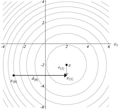
To illustrate the idea of conjugacy, the coordinate axes can be specified as search directions (Figure 2). The first step (horizontal) leads to the correct x coordinate of the solution x ∗ >^> . The second step (vertical) will reach the correct y coordinate of the solution x ∗ >^> and then finish searching. We define that the error e i = x ∗ − x i >_=>^->_> is a vector that indicates how far x i >_> is from the solution. The residual g i = b − A x i >_=>->_> indicates how far Ax i >_> is from the correct value of b <\displaystyle >> . Notice that e 1 >_> is orthogonal to d 0 >_> . In general, for each step we choose a point
.
To find the value of α i > , use the fact that e i >_> should be orthogonal to d i >_> so that no need to step in the direction of d i >_> again in the later search. Using this condition, we have
.
Then conduct transformation A > on both sides
So α k > can be obtained as the following:
.
Proof:
The error e 0 > from the starting point to the solution can be formulated as the following:
And the traversed steps from the starting point to the point x k >_> can be expressed as the following:
The residual term from the solution point to the point x k >_> can be expressed as the following:
Therefore, the α k > is as the following:
But, still, the solution x ∗ >^> has to be known first to calculate α k > . So, the following manipulations can get rid of using x ∗ >^> in the above expression:
The conjugate gradient method is a conjugate direction method in which selected successive direction vectors are treated as a conjugate version of the successive gradients obtained while the method progresses. The conjugate directions are not specified beforehand but rather are determined sequentially at each step of the iteration [4] . If the conjugate vectors are carefully chosen, then not all the conjugate vectors may be needed to obtain the solution. Therefore, the conjugate gradient method is regarded as an iterative method. This also allows approximate solutions to systems where n is so large that the direct method requires too much time [2] .
Set the maximum iteration n
A l g 2 : R e v i s e d a l g o r i t h m f r o m A l g 1 w i t h o u t p a r t i c u l a r c h o i c e o f D _ >>
Set the maximum iteration n
The formulas in the Alg 2 can be simplified as the following:
Then β i > and α i > can be simplified by multiplying the above gradient formula by g i >_> and g i − 1 >_> as the following:
This gives the following simplified version of Alg 2:
A l g 3 : S i m p l i f i e d v e r s i o n f r o m A l g 2 _ >>
Set the maximum iteration n
Consider the linear system A x = b >=>>
.
The initial starting point is set to be
.
Implement the conjugate gradient method to approximate the solution to the system.
Solution:
The exact solution is given below for later reference:
.
Step 1: since this is the first iteration, use the residual vector g 0 >_> as the initial search direction d 1 >_> . The method of selecting d k >_> will change in further iterations.
Step 2: the scalar α 1 > can be calculated using the relationship
Step 3: so x 1 >_> can be reached by the following formula, and this step finishes the first iteration, the result being an "improved" approximate solution to the system, x 1 >_> :
Step 4: now move on and compute the next residual vector g 1 >_> using the formula
Step 5: compute the scalar β 2 > that will eventually be used to determine the next search direction d 2 >_> .
Step 6: use this scalar β 2 > to compute the next search direction d 2 >_> :
Step 7: now compute the scalar α 2 > using newly acquired d 2 >_> by the same method as that used for α 1 > .
Step 8: finally, find x 2 >_> using the same method as that used to find x 1 >_> .
Therefore, x 2 >_> is the approximation result of the system.
Conjugate gradient methods have often been used to solve a wide variety of numerical problems, including linear and nonlinear algebraic equations, eigenvalue problems and minimization problems. These applications have been similar in that they involve large numbers of variables or dimensions. In these circumstances any method of solution which involves storing a full matrix of this large order, becomes inapplicable. Thus recourse to the conjugate gradient method may be the only alternative [5] . Here we demonstrate three application examples of CG method.
The conjugate gradient method is used to solve for the update in iterative image reconstruction problems. For example, in the magnetic resonance imaging (MRI) contrast known as quantitative susceptibility mapping (QSM), the reconstructed image χ is iteratively solved for from magnetic field data b >> by the relation [6]
Where D is the matrix expressing convolution with the dipole kernel in the Fourier domain. Given that the problem is ill-posed, a physical prior is used in the reconstruction, which is framed as a constrained L1 norm minimization
A detailed treatment of the function f ( χ ) and g ( χ ) can be found at [6] . This problem can be expressed as an unconstrained minimization problem via the Lagrange Multiplier Method
The first-order conditions require ∇ χ E ( χ , λ ) = 0 E(\chi ,\lambda )=0> and ∇ λ E ( χ , λ ) = 0 E(\chi ,\lambda )=0> . These conditions result in ∇ χ f ( χ ) + ∇ χ g ( χ ) − c ~ = 0 f(\chi )+\nabla _g(\chi )->=0> and ‖ g ( χ ) − c ‖ 2 2 ≈ ε ^\approx \varepsilon > , respectively. The update can be solved for ∇ χ f ( χ ) + ∇ χ g ( χ ) − c ~ = L ( χ ) χ − c ~ = 0 f(\chi )+\nabla _g(\chi )->=L(\chi )\chi ->=0> via fixed point iteration [6] .
And expressed as the quasi-Newton problem, more robust to round-off error [6]
Which is solved with the CG method until the residual ‖ χ n + 1 − χ ‖ 2 / ‖ χ n ‖ 2 ≤ θ -\chi \right\|_/\left\|\chi _\right\|_\leq \theta > where θ is a specified tolerance, such as 10 − 2 > .
Additional L1 terms, such as a downsampled term [7] can be added, in which case the cost function is treated with penalty methods and the CG method is paired with Gauss-Newton to address nonlinear terms.

The realization of face recognition can be achieved by the implementation of conjugate gradient algorithms with the combination of other methods. The basic steps is to decompose images into a set of time-frequency coefficients using discrete wavelet transform (DWT) (Figure 3) [8] . Then use basic back propagation (BP) to train a neural network (NN). And to overcome the slow convergence of BP using the steepest gradient descent, conjugate gradient methods are introduced. Generally, there are four types of CG methods for training a feed-foward NN, namely, Fletcher-Reeves CG, Polak-Ribikre CG, Powell-Beale CG, and scaled CG. All the CG methods include the steps demonstrated in Alg 3 with their respective modifications [8] [10] .
Notice that β k > is a scalar that varies in different versions of CG methods. β k > for Fletcher-Reeves CG is defined as the following:
where g i − 1 >_> and g i >_> are the previous and current gradients, respectively. Fletcher Reeves suggested restarting the CG after every n or n+1 iterations. This suggestion can be very helpful in practice [10] .
The second version of the CG, namely, Polak-Ribiere CG, was proposed in 1977 [11] . In this algorithm, the scalar at each iteration is computed as [12] :
Powell has showed that Polak-Ribiere CG method has better performance compared with Fletcher-Reeves CG method in many numerical experiments [10] .
The mentioned CGs, Fletcher-Reeves and Polak-Ribitre algorithms, periodically restart by using the steepest descent direction every n or n + 1 iterations. A disadvantage of the periodical restarting is that the immediate reduction in the objective function is usually less than it would be without restart. Therefore, Powell proposed a new method of restart based on an earlier version [10] [12] . As stated by this method, when there is negligibility orthogonality left between the current gradient and the previous gradient (the following condition is satisfied), the restart occurs [10] [12] .
Another version of the CG, scaled CG, was proposed by Moller. This algorithm uses a step size scaling mechanism that avoids a time consuming line-search per learning iteration. Moller [13] has showed that the scaled CG method has superlinear convergence for most problems.
The conjugate gradient method introduced hyperparameter optimization in deep learning algorithm can be regarded as something intermediate between gradient descent and Newton's method, which does not require storing, evaluating, and inverting the Hessian matrix, as it does Newton's method. Optimization search in conjugate gradient is performed along with conjugate directions. They generally produce faster convergence than gradient descent directions. Training directions are conjugated concerning the Hessian matrix.
Let’s denote d >> as the training direction vector. Starting with an initial parameter vector w 0 >_> and an initial training direction vector d 0 = − g 0 >_=->_> , the conjugate gradient method constructs a sequence of training direction as:
Here γ is called the called the conjugate parameter. For all conjugate gradient algorithms, the training direction is periodically reset to the negative of the gradient. The parameters are then improved according to the following expression:
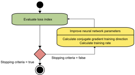
The training rate η is usually found by line minimization. Figure 4 depicts an activity diagram for the training process with the conjugate gradient. To improve the parameters, first compute the conjugate gradient training direction. Then, search for a suitable training rate in that direction. This method has proved to be more effective than gradient descent in training neural networks. Also, conjugate gradient performs well with vast neural networks since it does not require the Hessian matrix.


